improver.precipitation.precipitation_duration module

Module containing the PrecipitationDuration class.

class PrecipitationDuration(min_accumulation_per_hour, critical_rate, target_period, percentiles, accumulation_diagnostic='probability_of_lwe_thickness_of_precipitation_amount_above_threshold', rate_diagnostic='probability_of_lwe_precipitation_rate_above_threshold', model_id_attr=None)

Bases: PostProcessingPlugin

Classifies periods of precipitation intensity using a mix of the maximum precipitation rate in the period and the accumulation in the period. These classified periods are then used to determine what fraction of a constructed longer period would be classified as such. Percentiles are produced directly from these fractions via a frequency table. This is done to reduce the memory requirements when potentially combining so much data. The discrete nature of the fractions that are possible makes this table approach possible.

Note that we apply linear interpolation in the percentile generation, meaning that fractions of the target period that are not multiples of the input data period can be returned.

Percentile generation from a frequency table

Construction of the precipitation duration diagnostics involves a lot of input data. When working with a large ensemble, and constructing a long period from many short periods, the array sizes can become very memory hungry if operated on all at once. Every additional threshold that is included in the processing further exacerbates this issue. For example, input cubes something like this:

• realizations = 50

• times = 8 x 3-hour periods to construct a 24-hour target.

• number of combined rate and accumulation thresholds = 3

• y and x = 1000

means we are combining and collapsing two cubes of shape (50, 8, 3, 1000, 1000).

We work around this using slicing, breaking the data up into smaller chunks that can be read into memory one at a time, their contribution assessed, and then the data freed. However, if we need to save out the result of this processing in its expanded form, or use it directly to generate percentiles, we still need to hold all of the resulting data in memory unless we implement some kind of piecemeal writing to disk. An alternative is to construct a frequency table that retains counts of where the data falls and generate our percentiles from this table. As we are calculating fractions of a day that are classified as wet with this plugin, we have a discrete set of potential fractions, which makes this frequency table approach possible without any loss of precision.

The method used in this plugin is as follows:

1. Extract the requested rate and accumulation threshold cubes from the input cubes.

2. Combine the extracted cubes to form a single max rate and a single accumulation cube, each with a time dimension, as well a threshold dimension if multiple thresholds have been requested.

3. If we are working with scalar (single valued) threshold coordinates, escalate these to dimensions anyway so we can work with arrays with a consistent number of dimensions.

4. Arrange the dimensions into a specific order so we know that when we index these we are working with the expected dimensions.

5. Generate a tuple of tuples that describe all the different combinations of rate and accumulation thresholds to be combined together to classify the precipitation.

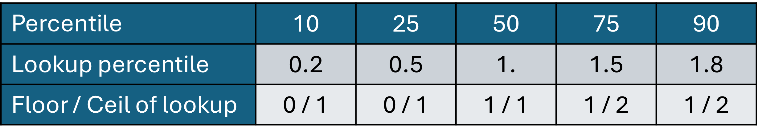
6. Scale the percentiles requested by the user to values in the range 0 to (realizations - 1). The table below shows an example, with 5 percentile values requested and these scaled to suitable lookup values for a 3-member ensemble (i.e. values of 0, 1 or 2).

7. Create a target array into which data will be placed. Note that if the number of percentiles being generated were as large as the number of realizations, we might not be doing much to reduce the memory with this approach.

8. Slice the data over the realization coordinate. We are therefore working with arrays with dimensions (threshold, time, y, x).

9. Realize the data by touching it, cube.data. This is done to reduce the amount of lazy loading of the data when we further subset it. Without this step the lazy loading and cleaning up of data takes much longer, making the plugin far too slow.

10. Loop over the different combinations of rate and accumulation thresholds. The inputs are binary probabilities, so we multiply them together to determine if a given location at a given time may be classified as precipitating by exceeding the rate and accumulation thresholds.

11. We sum over the time coordinate to get the total number of periods at each location that have been classified as precipitating.

12. As we are working with discrete periods we know all the values (number of periods) that could be returned by the sum over time. We use an array that has as one of its dimensions a length equal to this set of potential values. For each threshold combination and location we then add 1 into an array at an index in this dimension that corresponds to the value (number of periods) that was calculated. For example if a 24-hour period is being constructed from 3-hour period inputs, the possible values are between 0 (no periods classified) and 8 (all periods classified).

This table demonstrates how the hit count and cumulative table is formed for our example 3-member ensemble with data covering a 24-hour period in 3-hour chunks. The no of periods that can be classified as wet (8) determines the length of this array (shown here for a single grid cell). For each realization a value of 1 is added into the array at the index corresponding to the number of periods classified as wet. The hit count total is formed by summing across all realizations.

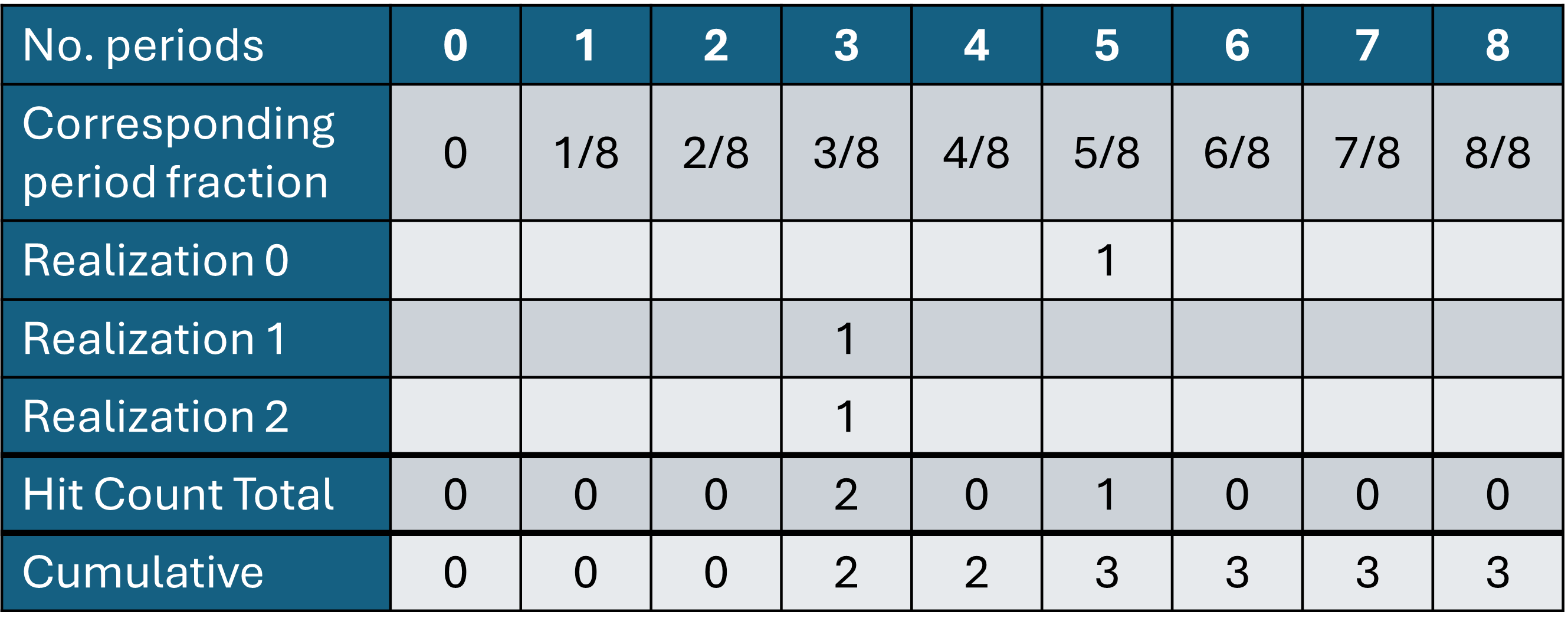
13. Once we have looped over all realizations we have a hit_count array of shape (accumulation_thresholds, rate_thresholds, N, y, x) where N corresponds to the possible number of periods. This is effectively a frequency table, telling us how many realizations, for each location, classified 0, 1, 2 etc. periods as precipitating. We loop again over the rate and accumulation thresholds and sum cumulatively along the periods dimension. The sum that’s returned is therefore a count of how many realizations classified each location as having fewer than or equal to n many periods classified as precipitating. This can be seen in the bottom row of the example table above.

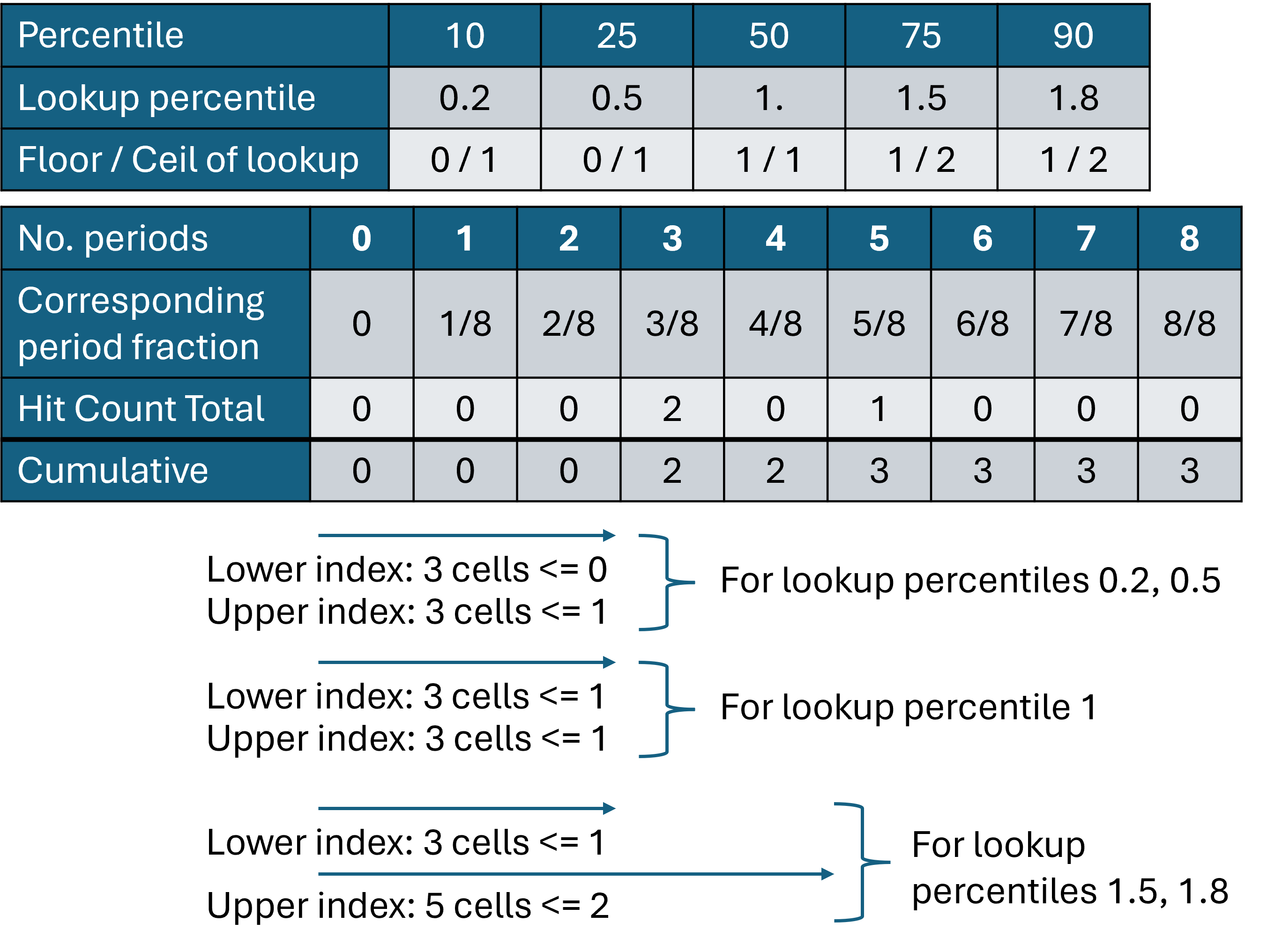
14. We can find the index in this cumulative list at which the various requested percentiles would fall. This allows us to get to the percentile we are after without having all of the values in hit_count represented individually in some array. The lower and upper bounds are found, i.e. our target percentile value sits between these two values.

This figure demonstrates the use of the cumulative table to lookup the bounding period fractions for our target percentile.

15. We perform a linear interpolation between the values to obtain our target percentile value. The interpolation fraction is the difference between the lookup percentile and the floored version of the same.

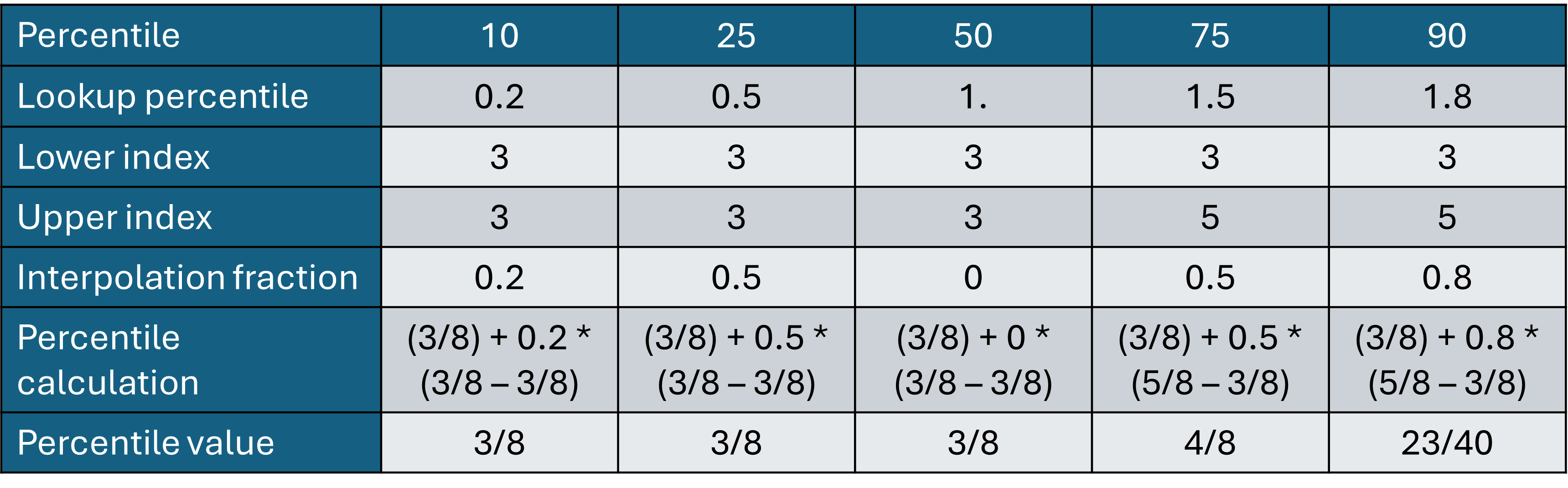
16. The calculated percentiles are stored for each combination of rate and accumulation thresholds and location, with these then written out to an output cube with suitable metadata.

__init__(min_accumulation_per_hour, critical_rate, target_period, percentiles, accumulation_diagnostic='probability_of_lwe_thickness_of_precipitation_amount_above_threshold', rate_diagnostic='probability_of_lwe_precipitation_rate_above_threshold', model_id_attr=None)

Initialise the class.

Parameters:

• min_accumulation_per_hour (float) – The minimum accumulation per hour in the period, or a list of several, used to classify the period. The accumulation is used in conjunction with the critical rate. Units of mm.

• critical_rate (float) – A rate threshold, or list of rate thresholds, which if the maximum rate in the period is in excess of contributes to classifying the period. Units of mm/hr.

• target_period (float) – The period in hours that the final diagnostic represents. This should be equivalent to the period covered by the inputs. Specifying this explicitly here is entirely for the purpose of checking that the returned diagnostic represents the period that is expected. Without this a missing input file could lead to a suddenly different overall period.

• percentiles (Union[List[float], ndarray]) – A list of percentile values to be returned.

• accumulation_diagnostic (str) – The expected diagnostic name for the accumulation in period diagnostic. Used to extract the cubes from the inputs.

• rate_diagnostic (str) – The expected diagnostic name for the maximum rate in period diagnostic. Used to extract the cubes from the inputs.

• model_id_attr (Optional[str]) – The name of the dataset attribute to be used to identify the source model when blending data from different models.

_abc_impl = <_abc._abc_data object>

_calculate_fractions(precip_accumulation, max_precip_rate, acc_thresh, rate_thresh, realizations, spatial_dims)

Calculate the fractions of the target period that are classified as wet using the given accumulation and peak rate thresholds. This is done by counting the number of periods in which the thresholds are exceeded out of the total number possible. Frequency tables are constructed and from these percentiles are calculated.

Parameters:

• precip_accumulation – Precipitation accumulation in a period.

• max_precip_rate – Maximum preciptation rate in a period.

• acc_thresh – Accumulation threshold coordinate.

• rate_thresh – Max rate threshold coordinate.

• realizations – A list of realization indices to loop over.

• spatial_dims – A list containing the indices of the spatial coordinates on the max_precip_rate cube, which are the same as for the precip_accumulation cube.

Raises:

ValueError – If the input data is masked.

Returns:

An array containing the generated percentiles.

static _construct_constraint(diagnostic, threshold_name, threshold_values)

Construct constraint to use in extracting the accumulation and rate data, at relevant thresholds, from the input cubes.

Parameters:

• diagnostic (str) – The name of the diagnostic to be extracted.

• threshold_name (str) – The name of the threshold from which to extract data.

• threshold_values (ndarray) – The threshold values to extract.

Return type:

Constraint

Returns:

Iris constraint to extract the target diagnostic and threshold values.

_construct_thresholds()

Converts the input threshold units to SI units to match the data. The accumulation threshold specified by the user is also multiplied up by the input cube period. So a 0.1 mm accumulation threshold will become 0.3 mm for a 3-hour input cube, converted to metres.

Return type:

Tuple[ndarray, ndarray]

Returns:

Tuple of float values, one the accumulation threshold, the other the rate threshold.

_create_output_cube(data, cubes, acc_thresh, rate_thresh, spatial_dim_indices)

Create an output cube for the final diagnostic, which is the set of percentiles describing the fraction of the constructed period that has been classified as wet using the various accumulation and peak rate thresholds.

Parameters:

• data (ndarray) – The percentile data to be stored in the cube.

• cubes (Tuple[Cube, Cube]) – Cubes from which to generate attributes, and the first of which is used as a template from which to take time and spatial coordinates.

• acc_thresh (DimCoord) – The accumulation threshold to add to the cube.

• rate_thresh (DimCoord) – The rate threshold to add to the cube.

• spatial_dim_indices – Indices of spatial coordinates on the the input cubes. This allows us to select the correct dimensions when handling either gridded or spot inputs.

Return type:

Cube

Returns:

A Cube with a suitable name and metadata for the diagnostic data stored within it.

_extract_cubes(cubes, diagnostic, threshold_name, threshold_values)

Extract target diagnostics and thresholds from the input cube list. Merge these cubes into a single cube with a multi-valued time dimension.

Parameters:

• cubes (CubeList) – The input cubes from which to extract targets.

• diagnostic (str) – The diagnostic name.

• threshold_name (str) – Name of the threshold coordinate from which to extract specific values.

• threshold_values (ndarray) – The threshold values to extract.

Raises:

ValueError – If the target diagnostic or thresholds are not found.

Returns:

The merged cube containing the target thresholds.

Return type:

cube

_period_in_hours(cubes)

Get the periods of the input cubes, check they are equal and return the period in hours. Sets the period as a class variable.

Parameters:

cubes (CubeList) – A list of cubes.

Raises:

ValueError – If periods of all cubes are not equal.

Return type:

None

static _structure_inputs(cube)

Ensure threshold and time coordinates are promoted to be dimensions of the cube. Ensure the cube is ordered with realization, threshold, and time as the three leading dimensions.

Parameters:

cube (Cube) – The cube to be structured.

Returns:

The reordered cube and the threshold coordinate.

Return type:

Tuple containing

process(*cubes)

Produce a diagnostic that provides the fraction of the day that can be classified as exceeding the given thresholds. The fidelity of the returned product depends upon the period of the input cubes.

This plugin can process an awful lot of data, particularly if dealing with a large ensemble. To reduce the memory used, given the discrete nature of the period fractions produced, frequency bins are used to directly produce percentiles. This means that not all of the values need to be held in memory at once, instead we count instances of each value and then calculate the percentiles from the counts.

Parameters:

cubes (Union[Cube, CubeList]) –

Cubes covering the expected period that include cubes of:

precip_accumulation: Precipitation accumulation in a period. max_precip_rate: Maximum preciptation rate in a period.

Return type:

Cube

Returns:

A cube of percentiles of the fraction of the target period that is classified as exceeding the user specified thresholds.

Raises:

• ValueError – If the input cubes have differing time coordinates.

• ValueError – If the input cubes do not combine to create the expected target period.

• ValueError – If the input cubes lack a realization coordinate.

• ValueError – If the input cubes have differing realization coordinates.